Smooth movements with Axis positioning units

Positioning cameras and positioning units from Axis offer smooth pan and tilt movements thanks to sophisticated motor control. The smoothness of camera movement is quantified using the standard deviation of the velocity, calculated at low speed. In Axis positioning cameras and positioning units, this has been measured to be less than ±0.01°/s. This variation is so small that the camera movements are perceived as jerk free.

Positioning cameras and positioning units from Axis offer smooth pan and tilt movements. Both when moving ultra-slow for panoramic viewing, or with high speed for instant pinpointing of a detected incident, the camera’s or positioning unit’s panning and tilting movements are uniform and free from visible jolting or shaking.

This white paper explains how Axis measures smoothness in movement, and why that method was chosen. It also details how velocity variations affect the viewing experience. Because the smoothness, or rather, the jerkiness, is quantified as a standard deviation, the last section describes the definition and calculation examples of that measure.

At Axis, the smoothness of camera movement is quantified using the standard deviation of the velocity, calculated at low speed. Standard deviation is a commonly used and proven way for computing how much a set of data values vary from a nominal value.

The standard deviation of the velocity has been measured to be less than ±0.01°/s in Axis positioning cameras. This variation is so small, thanks to sophisticated motor control, that the camera movements are perceived as jerk free.

Consider a camera panning, with low velocity, over a stationary object. If the velocity is constant, the object will appear to move an equal distance on the screen between every frame. The object will always show where you expect it to, that is, as predicted from previous frames.

If the camera panning velocity is not entirely constant, but instead jerky at the end, the object will appear to move a non-equal distance between frames, and seemingly make a jump to another place than where expected.

A larger velocity variation (larger amplitude) will be more noticeable, and a longer duration of the variation will be more visually disturbing. Standard deviation is defined to emphasize such variations, making it a very suitable method to quantify the jerkiness.

When observing a moving object, a camera can be set to keep the object constantly centered in the image. In that case, camera velocity variations will prevent the object from staying centered. The erratically moving background will also cause a visual disturbance that adds to the perceived level of jerkiness.

Different types of velocity variations can occur in camera movements:

Standard deviation is a commonly used and proven measure for quantifying how much a set of data values vary from a nominal value. The standard deviation is usually represented by lower-case σ (sigma).

The standard deviation of a set of data values is defined as:

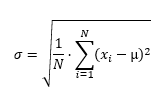
where σ is the standard deviation, x_i are the data values, µ is the mean value, and N is the number of data values. Note that a slightly different definition can be used if the data values are part of a larger number of samples. Step by step, the calculation can be done as follows. For reference, see the diagrams below, where data samples, mean value, error, and standard deviation are marked.

1. Calculate the mean of the data values.

2. For each data value, calculate the error as the difference between the data value and the mean value.

3. Take the square of each error. This makes all errors positive so that they do not cancel out, and it puts more emphasis on large errors.

4. Take the mean of the squared errors. This is the variance, σ².

5. Take the square root of the variance to get the standard deviation.

For a visualization of how the standard deviation correlates directly to the variation in values, compare the examples below where σ=1, σ=2, and σ=0.5.